


Reliable RTK depends on two things working together: a dense, high-quality reference network and a model that turns the data from that network into corrections that hold up under real conditions. Most providers will tell you about the density of their stations, fewer about their quality. Far fewer again will tell you what they do with the data from it. Skylark’s atmospheric model is the difference between corrections that usually work and corrections that work when applications usually break.
A robotic mower drifts 8 centimeters and lands in the flowerbed. An automated line painter draws a crooked stripe on a freshly paved road. An autonomous vehicle drifts into the oncoming lane.
None of these failures happen at the median of your error distribution. They happen at the tail, in the moments when the atmosphere stops cooperating. At scale, there is nowhere to hide. With enough devices in the field, the tail stops being a statistical edge case and becomes something every customer encounters during the product’s lifetime. That’s what every serious RTK provider competes on, and atmospheric modeling is the part of the system that decides what your customers actually experience there.
What atmospheric modeling actually does
GNSS signals get distorted as they pass through the upper atmosphere. The ionosphere bends them, the troposphere slows them, and both layers shift and reshape across space and time. The GNSS corrections must also remove satellite clock, orbit, and bias errors, but those are well-characterized. The atmosphere is the hard one.
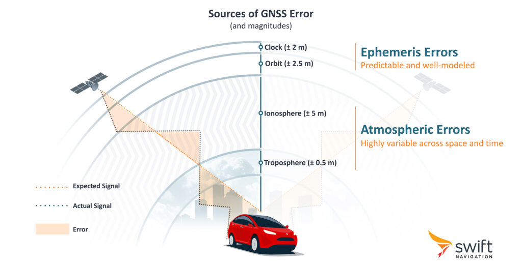
The basic way to handle this is to use a single nearby base station and assume the atmosphere over you matches the atmosphere over the base. That’s single-baseline RTK, and it works when conditions are calm and the user stays within roughly 20 kilometers of the base. When it moves farther away, or when conditions get turbulent, the assumption breaks and accuracy degrades. Any problems with the station performance or availability directly affects the user.
Scaling up to a network of stations and using geometric interpolation between them helps. However the corrections at the user location are still estimates based on the same limited assumptions, not physics.
The more powerful way is to build a model of the atmosphere itself. Instead of asking what a station miles away sees, you ask exactly what the ionosphere is doing along the satellite signal paths, and precisely correct for it.
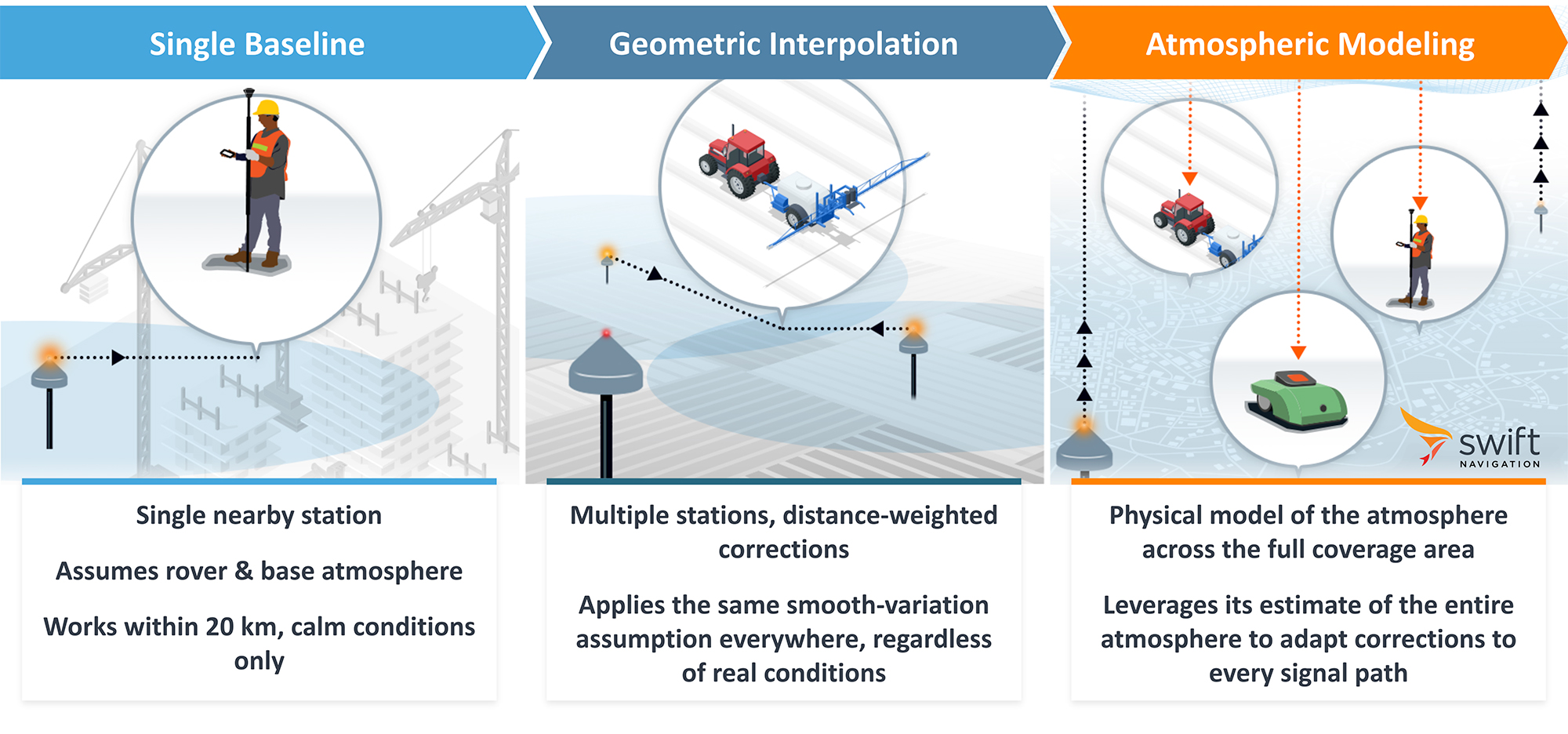
Combined with a high quality network, the model captures more than what sits between stations. It’s a physical representation of how electron density behaves in the layers above the Earth, fit to observations from every station in the network at every epoch. From that, it can predict the atmospheric state accurately at any point between stations. The model also tracks its own accuracy in real time. When conditions degrade, it can provide integrity information: how much error to expect, and whether the correction meets the safety requirements of the application.
Skylark has been built around atmospheric modeling from the beginning. From station hardware to correction delivery, every layer is purpose-built for precise, robust, and available GNSS corrections.
The 99th percentile is where modeling earns its keep
A dense reference network samples the atmosphere at high resolution. Helpful, but never enough on its own. The disturbances that cause the worst RTK fix problems happen at scales finer than any commercial network can sample directly. What matters is what the model estimates about the variation in between. Pure geometric interpolation assumes the atmosphere changes smoothly between any two stations. Most of the time that’s roughly true. During a traveling ionospheric disturbance or a magnetic storm, it isn’t, and that’s exactly when applications need their corrections to hold.
A single-baseline system has no defense against these events. The ionospheric error between rover and base passes straight through to the position solution. Geometric interpolation across a dense network does better by combining observations from multiple stations. But the correction at the rover still relies on the assumption that the atmosphere varies smoothly between them. When it doesn’t, errors leak through.
Skylark’s atmospheric model goes further. It acts as an elastic buffer: by modeling the ionosphere continuously in time and space, it absorbs the bulk of the storm-induced delay before it reaches the rover, typically around 95%. It also tracks disturbances as they propagate: a wave that hit one station two minutes ago is likely arriving at the next one now, and the model stays ahead of it.
These conditions also expose a subtler problem. RTK engines are sensitive to outliers: even one or two satellite signals carrying large ionospheric errors can corrupt the fix. Neither single-baseline nor geometric interpolation can reliably identify which signals are compromised at the rover’s location. Skylark can: when the model flags lines of sight with anomalously large residuals, those satellites can be excluded from the solution. The rover only uses clean data.
Stations and modeling are multiplicative
A useful analogy: cameras and image quality. A 48-megapixel sensor on its own still produces worse photos in low light than a 12-megapixel sensor paired with quality optics and image processing. Resolution alone doesn’t get you a great photograph. The pipeline matters: how the sensor handles noise, how the firmware fuses exposures, how the system reasons about what it’s actually looking at.
A reference network is megapixels. Atmospheric modeling is the imaging pipeline. The two compound, and investing in one without the other leaves performance on the table. But they don’t scale the same way.
The brute force tax
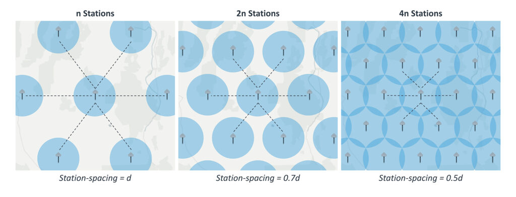
There’s also a practical reality to building RTK at scale: station density alone is a brute force lever, and the math punishes it fast. If you double your station count, you only shrink station spacing by 30 percent, because you’re sampling in two dimensions. To halve the spacing, you need to quadruple the station count. The returns diminish fast.
This is when providers start cutting corners: lower-quality hardware, noisier RF environments, less resilient connectivity, infrequent maintenance, and stations deployed in less ideal locations with nearby obstructions. Building a dense network is one challenge. Maintaining it at scale is another. If operations teams do not scale alongside the network, a meaningful percentage of stations inevitably ends up degraded or offline. A correction service is only as good as the station data going in. Coverage looks great on a map, but performance suffers, especially at the tail.
No boundaries, no jumps
The model represents the atmosphere as one continuous field across the coverage area, abstracting the underlying network of stations. A rover gets a unified prediction at any point, not a localized correction handed off between bases, so the positioning jumps that come with crossing station boundaries in traditional Network RTK simply don’t exist.
When a station drops, the model holds
This follows from that same abstraction. When a station drops out of a model-based service, the system loses one input among many. When a station drops out of a station-centric service, an entire sector of coverage drops with it.
Integrity by design
Because the model produces an uncertainty estimate alongside every correction, downstream systems can make integrity decisions in real time, not just consume corrections and hope. This is part of what enabled Skylark to become the first cloud-based real-time corrections service certified to ISO 26262, the automotive functional safety standard.
This is why the largest commercial deployments in this category, the ones serving autonomous vehicles and continent-scale fleets, lean on modeling rather than trying to achieve uniform density across Wyoming, rural Spain, or Hokkaido. The model is doing real work in places where stations alone would never reach the right answer. That’s most of the planet.
One model. Three delivery formats.
Skylark comes in three variants. They look different from the outside. Inside, they leverage the same atmospheric model.
- Skylark Nx RTK delivers VRS-formatted corrections for standard RTK receivers, with 1 to 2 centimeter accuracy. The classic RTK use case: surveying, precision agriculture, precision robotics, micromobility compliance.
- Skylark Cx delivers PPP-RTK via OSR and SSR corrections for continent-scale coverage with no baseline dependence, at 3 to 7 centimeter accuracy. Designed for automotive, fleet workloads, autonomous mobile robotics, and any application where safety is paramount.
- Skylark Dx delivers DGNSS for sub-meter use cases. Lowest power and bandwidth consumption. Ideal for IoT, small trackers, and mobile devices.
Swift’s atmospheric model sits upstream of all three. The variant a customer picks is a question of delivery format, receiver capability, and what the application needs. The modeling is the same.
For customers building products that have to scale, that matters. A consumer pet tracker, a delivery robot, and a tractor can all run on the same underlying infrastructure with the right delivery format for each.
What the model looks like under the hood
For the technically curious: at its heart, the Skylark atmospheric model leverages advanced spatial machine learning rooted in Gaussian Process theory. The model dynamically adapts to changing GNSS atmospheric conditions by continuously training on data from Swift’s global reference network.
The training data now spans nearly a decade and a full solar cycle, and includes fault-injected and historical event data, so the model has seen the conditions that matter most: geomagnetic storms and atmospheric anomalies. It captures the complex spatial and temporal relationships in the ionosphere and troposphere across a very large parameter space, and keeps refining as new data flows in.
The model is constrained by physics-based rules governing how the atmosphere actually behaves. It represents the ionosphere as a stack of thin shells at the altitudes where electron density peaks, and captures the actual path of each GNSS signal through individual ionospheric layers. Physical limits bound spatial gradients and temporal evolution. The model solves for receiver and satellite biases alongside the atmospheric state, and rejects outlier observations through a robust consensus algorithm. ML-based algorithms continuously monitor ionospheric conditions, detecting disturbances in real time. The result is a model that produces physically consistent solutions, not just statistically plausible ones.
In plain language: physics where physics works, machine learning where physics needs help. The model runs at continental scale and produces both a correction and a measure of its own confidence in that correction.
How to evaluate a corrections provider
Spec sheets are written to sound impressive. Here’s what to actually look for.
| What to evaluate | What to look for |
|---|---|
| The network in your specific operating regions | Per-region station density (not the global average), redundancy at each site (dual antennas and receivers, backup power, multiple backhaul paths), and a published SLA with real accountability. A station map is table stakes; the operations infrastructure behind it is what matters. |
| The model itself, not just the data feed | A serious provider can explain how the atmospheric state is estimated and how the system behaves during active ionospheric conditions. Replay data from storm days is more telling than calm-day demos. |
| Tail performance, not headline accuracy | 99th percentile accuracy under representative conditions, not just median or 95th. The tail is what determines whether your application is robust or will break. |
| Geographic scalability | Coverage in the regions you’ll need next year and the year after. A service that depends solely on uniform high station density everywhere doesn’t scale to the geographies most production deployments reach. |
| The receiver side | The receivers the provider has validated with, whether the service requires their own brand of hardware, and how performance degrades when rover hardware is less capable than the reference hardware in their test data. |
The bottom line
Reliable RTK has two ingredients: a high-quality reference network, and modeling that gets the most out of it. Both are real engineering problems, and both deserve real investment. Swift has built both: dense reference networks in every market we serve, and the atmospheric model that has been running in production for nearly a decade.
The deciding factor between corrections that work most of the time and corrections that work all of the time is what happens when the atmosphere doesn’t behave like an average day. That’s the problem Skylark was built around, and where we keep pushing the baseline.