What is Ionospheric Delay?
Ionospheric delay is the slowing of GNSS satellite signals as they pass through the ionosphere — the layer of Earth’s atmosphere from approximately 60–1,000 km altitude — where solar radiation ionises gas molecules into free electrons. These free electrons slow the GNSS signal code (while advancing the carrier phase), causing a receiver to overestimate its distance from the satellite and producing positioning errors of up to 5–10 metres during peak solar activity.
What Causes Ionospheric Delay?
The ionosphere contains a plasma of electrically charged particles (free electrons) created when solar UV and X-ray radiation strips electrons from atmospheric gas molecules. GNSS signals interact with this plasma in two ways:
- Group delay (code slowing): The signal’s modulation travels slower than in a vacuum, producing an artificially long measured travel time and a positive range error.
- Phase advance: The carrier wave phase travels faster through the ionosphere — creating equal and opposite effects on code and carrier measurements. Dual-frequency receivers exploit this relationship to cancel the delay.
The magnitude of delay depends on Total Electron Content (TEC) — the integrated density of electrons along the signal path. TEC varies with solar activity, time of day, season, geographic latitude, and the phase of the 11-year solar cycle.
The extent of this delay depends on factors like the angle at which the satellite signal enters the ionosphere (satellite elevation angle) and the Total Electron Content (TEC) – the total number of electrons – along the signal’s path. TEC varies with solar activity, time of day, season, geographic latitude, and the phase of the 11-year solar cycle. Total Electron Content is a key measure of ionospheric activity, and models like the Single Layer Model (SLM), which treats the ionosphere as a thin shell at about 400 km altitude, help convert these delays for practical use.
How Large is the Ionospheric Error?
At vertical incidence, ionospheric delay typically introduces 1–10 metres of equivalent range error. At low elevation angles, signals travel longer paths through the ionosphere, amplifying the delay by 3–5×.
- Nominal mid-latitude daytime: 2–5 m horizontal position error from ionospheric delay alone.
- Solar storm or equatorial scintillation: Up to 30–50 m range error; standard correction models may fail.
How Ionospheric Delay is Corrected
- Dual-frequency receivers: Because ionospheric delay is frequency-dependent, tracking two frequencies (e.g., L1+L5) allows the receiver to compute and cancel ~99% of the delay without any external data. Learn more about dual frequency GNSS in our blog L1/L2 vs L1/L5: Evaluating Dual-Frequency GNSS for High Precision Applications.
- Broadcast ionospheric models: GPS broadcasts the Klobuchar model; Galileo broadcasts the NeQuick model. These reduce ionospheric error by ~50% for single-frequency receivers.
- SBAS: Ground networks measure TEC and broadcast wide-area ionospheric corrections, reducing error to <1 m for single-frequency receivers.
- RTK / Network RTK: Nearby reference stations experience nearly the same ionospheric delay as the rover. Differencing cancels the common error. Network RTK models the spatial variation of ionospheric delay across a wide area.
- PPP-RTK SSR maps: Regional ionospheric delay maps are sent to the receiver, enabling fast convergence without a nearby base station.
The impact of ionospheric delay can vary significantly. Therefore, high-precision GNSS systems often include quality control measures, such as setting thresholds for acceptable delay values, and may exclude data that falls outside these limits to maintain accuracy.
For demanding applications requiring precise positioning, effectively handling ionospheric delays is critical. Modern multi-constellation receivers leverage signals from various satellite systems and frequencies to improve their estimation and compensation of these delays. This leads to more reliable and accurate GNSS performance, particularly in challenging environments where ionospheric effects might be more pronounced. Continuous monitoring and correction of ionospheric delays are essential for consistent and accurate GNSS operation across diverse use cases.
How Swift Navigation models ionospheric delay
Skylark's atmospheric model uses machine learning combined with physics-based constraints to model ionospheric delay in real time — maintaining correction accuracy even during geomagnetic storms and challenging equatorial conditions.
Read: Atmospheric Modelling in GNSS Corrections →Frequently Asked Questions
No. Ionospheric delay varies significantly with time of day (peaks in the afternoon), season, solar cycle phase, and geographic location. Solar flares and geomagnetic storms can cause sudden, severe increases that are difficult to model in real time.
Yes — ionospheric delay affects all satellite signals passing through the ionosphere similarly. However, receivers tracking more constellations have more satellites at varied geometries, reducing the overall impact. Newer signals, such as Galileo's E5 signal, have properties that make it less susceptible to scintillation effects.

A single-frequency receiver cannot self-calibrate ionospheric delay and must rely on broadcast models or external corrections (SBAS, RTK, PPP-RTK). For precision applications requiring centimetre accuracy, a dual-frequency receiver with RTK corrections is strongly recommended.

Related Glossary Terms
Related Content
GNSS Basics
Marwan Ramadan
Devon Sharp
Marwan Ramadan
Marwan Ramadan
Devon Sharp
Devon Sharp
Marwan Ramadan
Devon Sharp
GIS
Devon Sharp
ROBOTICS
Marwan Ramadan
Emilee Pierce